How To: Perform a Nested Analysis

We're really excited to make our popular Nested tool freely available online - if you're interested in why we're giving this away free of charge, then please read our blog to learn more!

In this overview of the tool, we’ll use a case study to illustrate how to use it and how to interpret the output. This example comes from a manufacturing background, and records the particle size distribution (D50) measurement of a formulation product. In a perfect world, every measurement would yield the same result - but, in reality, we know that results will vary, and we'd like to understand why.

We'll look at this process across 4 batches, taking two samples from each batch. We'll then measure each sample twice, and record the results. If you'd like to download the sample data to try it out for yourself, then you can do so here. This file will show the required layout for a Nested analysis - one row per measurement, with one column per factor and response.

First things first: let's import the data. You can either load a CSV into the website, or copy and paste the data directly from Excel. If you're concerned about the risks of putting your data onto our website, then we hope that our "How secure is my data?" blog will address your concerns.

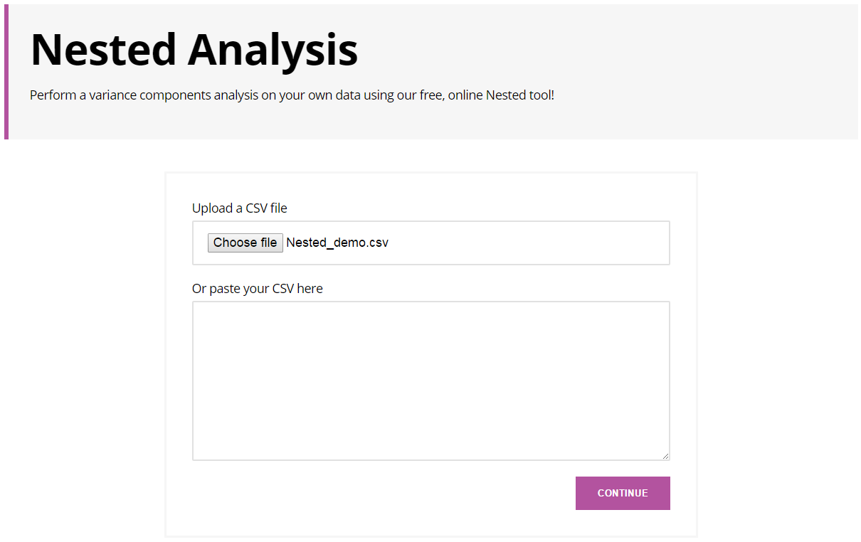
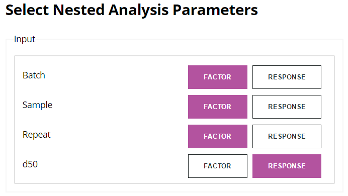
You then need to define the column roles and analysis parameters. Set Batch, Sample and Repeat as Factors, and d50 as your Response.

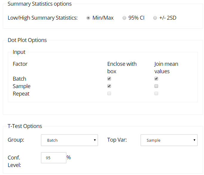
You can then set your analysis parameters - we'll leave these at the default settings for the time being, but feel free to try out the various options:

After clicking Continue, you'll be presented with the analysis results. The first section allows you to define the Lower and Upper Specification Limits (LSL and USL), as well as specifying the factors into the commonly-used ICH categories of Reproducibility, Intermediate Precision and Repeatability. If you want to enter or change these values, do so now.

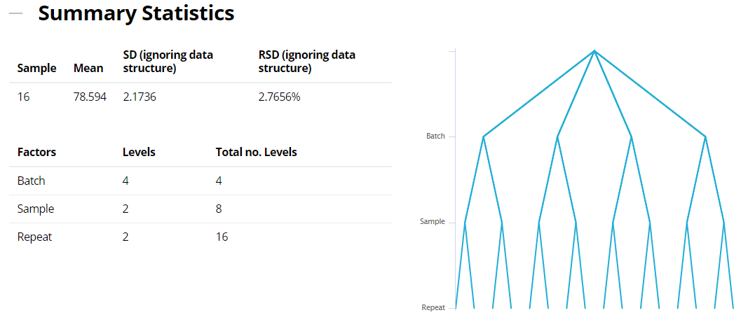
We can then drill down into the output, where each report section can be hidden or displayed using the - and + icons. The first section provides you with some Summary Statistics, listing the sample size and overall mean and SD. It also lists the various factors, along with the number of levels detected for each one. Finally, a diagram is provided to give you an overview of your dataset's structure.

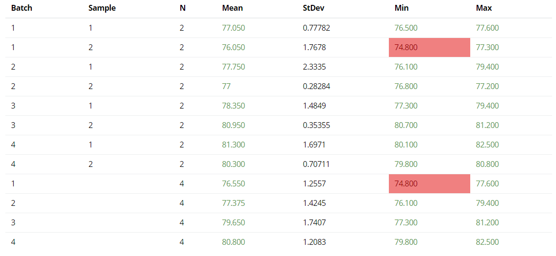
Further statistics are then produced for each combination of factor settings. Depending on your selection in the "Low/High Summary Statistics" analysis option, you'll be presented with either the Min/Max, 95% Lower/Upper Confidence Intervals or Mean +/- 2SD. If you entered LSL and/or USL values, then any values that fall outside these limits are colour-coded red.

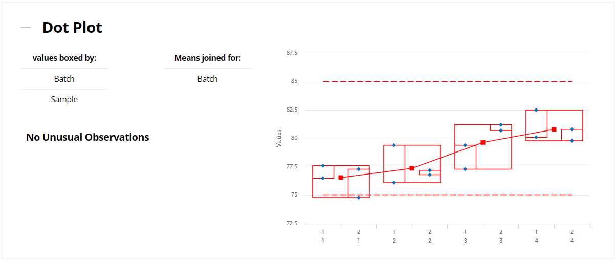
Next, you'll find the Dot Plot section. This provides a visual representation of the individual results, and in this example the values are boxed by the four Batches, and then by the two Samples within each Batch. The mean values for each Batch are also plotted, and joined with a line - this shows a drift upwards across the four Batches. If you'd like to create a box or join mean values for different factors, then you can do this via the "Dot Plot Options" on the analysis parameters. The LSL and USL are also displayed (if defined), and if there are any potential outliers detected then these are listed and colour-coded red on the graph.

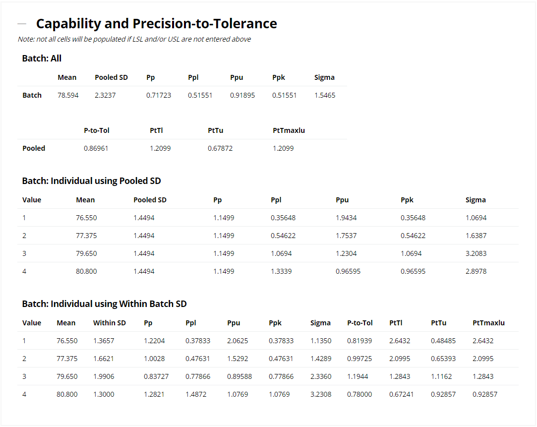
Capability and Precision-to-Tolerance provides a number of metrics that indicate how variable the process is, relative to specification. Most of these values can only be calculated if LSL and/or USL are defined. Capability metrics (such as Ppk and Sigma) and Precision-to-Tolerance are generated, using both a pooled estimate of variation as well as looking at the individual Batches separately.

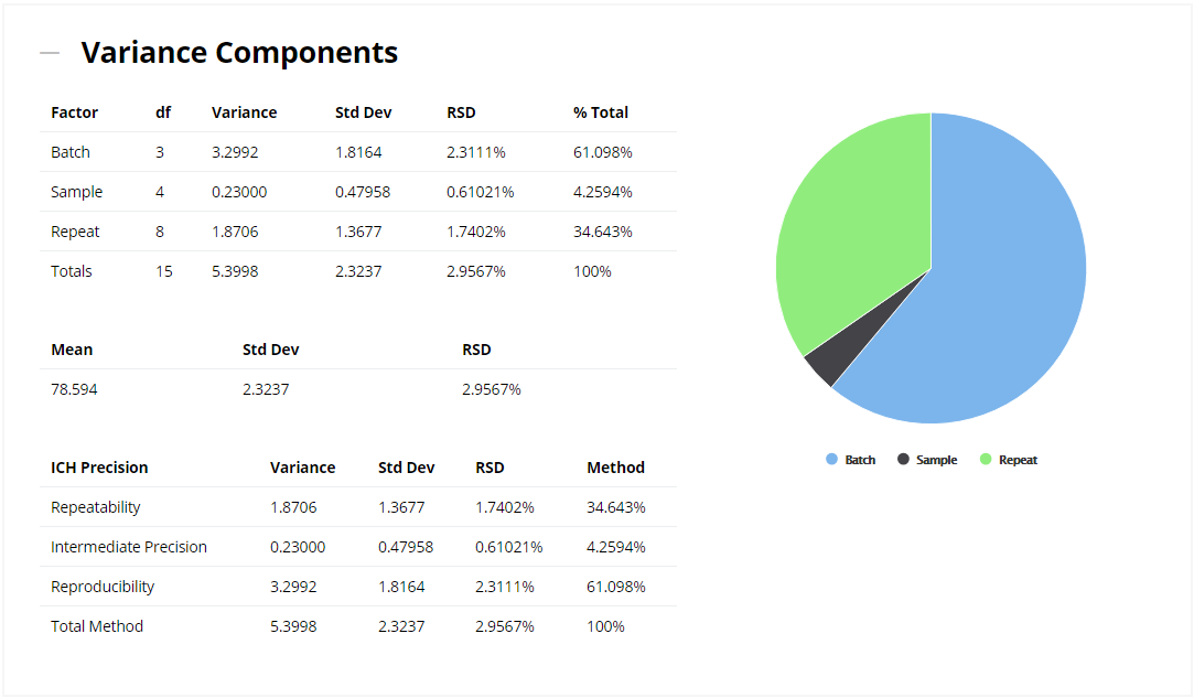
The Variance Components section contains perhaps the most useful information: which factors are causing the largest amount of variation. We're generally interested in reducing variation as much as possible, and the first table and pie chart show that over 60% of the total variation is caused by Batch-to-Batch changes. If we can find a way to make our Batches more consistent, then this will have a large impact on reducing the overall noise. A very small proportion of the total variation is caused by Sample, suggesting that these are consistent throughout the production run of a Batch. However, over 30% of the total variation comes from Repeat measurements of the same sample! This might point us towards ensuring our equipment is correctly calibrated and sufficiently precise, and that all of our analysts are following the same SOPs. 

This section also lists the Mean, Standard Deviation (accounting for the data structure) and Residual Standard Deviation (a.k.a. Coefficient of Variation, or CV). Finally, the variance components are grouped into the ICH categories defined in the Analysis Parameters section.

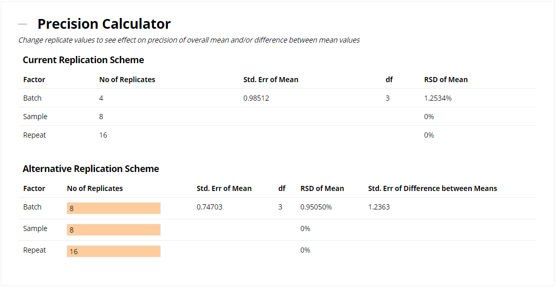
The Precision Calculator allows you to compare your existing replication scheme with an alternative one, helping you to identify where you'll achieve the greatest improvement in precision. Try out various "what if?" scenarios by entering values in the input cells.

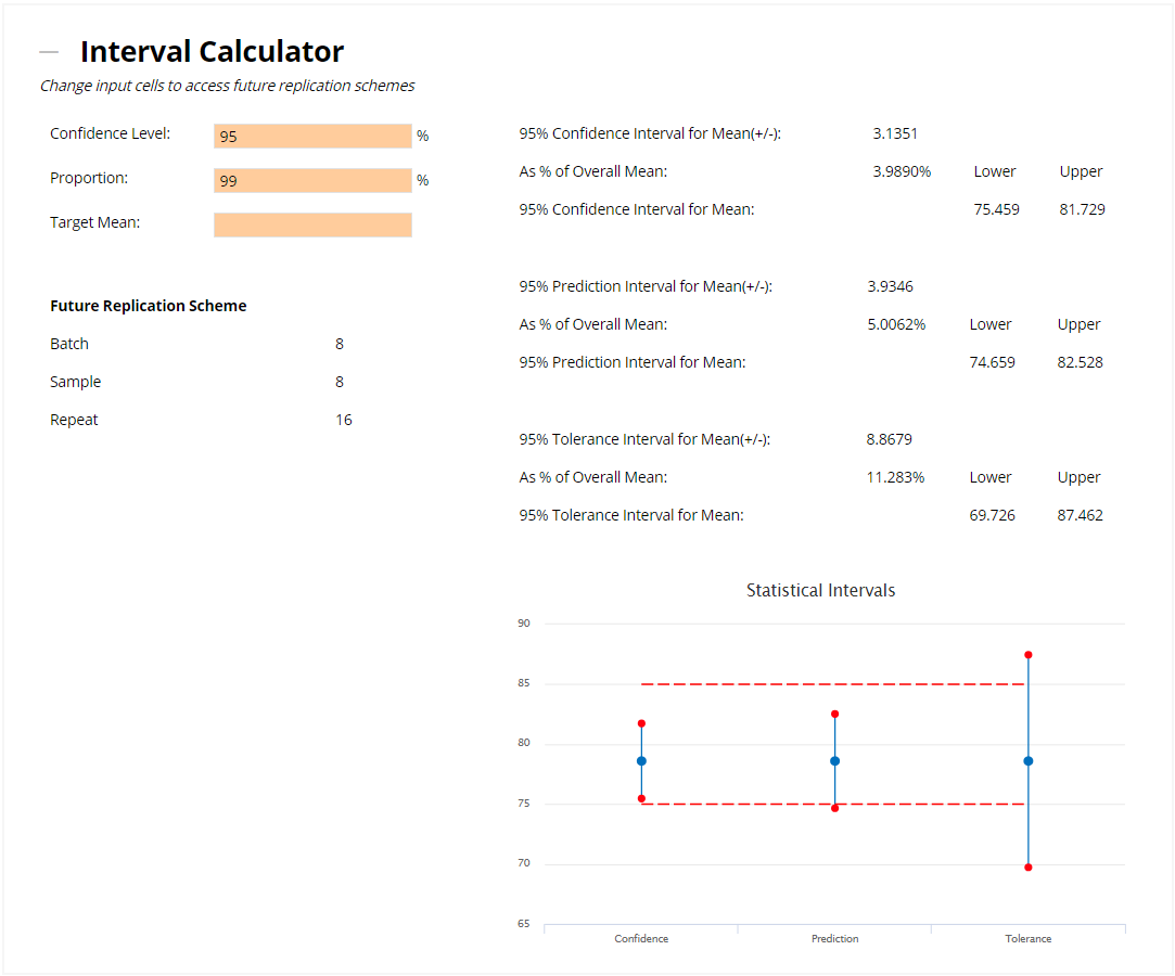
The values entered in the Alternative Replication Scheme above are then fed into the Interval Calculator, which displays the Confidence, Prediction and Tolerance Intervals around the overall mean value. You can set the Confidence Level for the CI, PI and TI, as well as the Proportion for the TI. Finally, if you'd rather base the intervals around a target value (rather than the calculated mean of the dataset), then you can enter a Target Mean as well. If you defined the LSL and/or USL earlier, then these limits will be plotted on the graph.

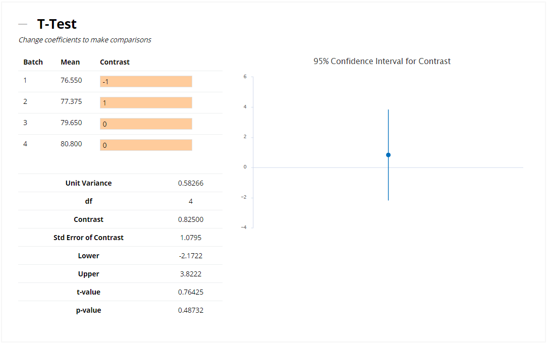
The final section allows you to compare Batches against one another, using the T-Test. You can contrast your chosen Batches by entering -1 and +1 in the input cells, and this will then perform a t-test to determine whether they are statistically significantly different from one another - if they are, then the p-value will be less than 0.05 and the 95% Confidence Interval (displayed on the graph, and listed as Lower and Upper) will not include zero. In the following example, Batches 1 and 2 are not statistically significantly different. If you'd prefer to compare levels of a different factor (e.g. Sample) or use a different confidence level, then you can specify this in the "T-Test Options" of the analysis parameters.